helita

Helita documentation can be found here (the installation section is taken from this link):

http://helita.readthedocs.io/en/latest/index.html

Helita is a Python library for solar physics focused on interfacing with code and projects from the Institute of Theoretical Astrophysics (ITA) at the University of Oslo. The name comes from Helios + ITA. Currently, the library is a loose collection of different scripts and classes with varying degrees of portability and usefulness.

---

Installation

Pre-requisites

To make use of helita you need a Fortran compiler (GFortran is recommended), because some modules are compiled from Fortran. The packages in the left column should be installed before installing helita. The right column contains recommended packages that allow the user to take advantage of all of the features.

Required	Recommended
Python (2.7.x, 3.4.x or later) Astropy NumPy SciPy	Matplotlib h5py netCDF4 Cython pandas beautifulsoup4

Helita will install without the recommended packages, but functionality will be limited. All of these packages are available through Anaconda, and that is the recommended way of setting up your Python distribution.

Cloning git repository

The easiest way is to use git to clone the repository. To grab the latest version of helita and install it:

$ git clone https://github.com/ITA-solar/helita.git
$ cd helita
$ python setup.py install

Note

The majority of the most updated versions of bifrost.py, ebysus.py, and all things bifrost related are in the https://github.com/jumasy/helita.git fork.

Non-root install

If you don’t have write permission to your Python packages directory, use the following option with setup.py:

$ python setup.py install --user

This will install helita under your home directory (typically ~/.local)

Developer install

If you want to install helita but also actively change the code or contribute to its development, it is recommended that you do a developer install instead:

$ python setup.py develop

This will set up the package, such as the source files used, from the git repository that you cloned (only a link to it is placed on the Python packages directory). Can also be combined with the -user flag for local installs:

$ python setup.py develop --user

Installing with different C or Fortran compilers

The procedure above will compile the C and Fortran modules using the default gcc/gfortran compilers. It will fail if these are not available in the system. If you want to use a different compiler, please use setup.py with the -compiler=xxx and/or -fcompiler=yyy options, where xxx, yyy are C and Fortran compiler families (names depend on system). To check which Fortran compilers are available in your system, you can run:

$ python setup.py build --help-fcompiler

and to check which C compilers are available:

$ python setup.py build --help-compiler

---

bifrost.py

bifrost.py is a set of tools to read and interact with output from Bifrost simulations. LMSAL has also contributed to this.

BifrostData class

bifrost.py includes the BifrostData class (among others). The following allows to create the class for snapshot number 430 from simulation ‘cb10f’ from directory ‘/net/opal/Volumes/Amnesia/mpi3drun/Granflux’ (a network local to LMSAL):

from helita.sim import bifrost as br

dd = br.BifrostData('cb10f', snap = 430, fdir = '/net/opal/Volumes/Amnesia/mpi3drun/Granflux', verbose = False)

The snapshot(s) being read can be defined when creating the object, or set/changed anytime later. Snaps can be ints, arrays, or lists.

Getting variables & quantities

get_var and get_varTime can be used to read variables as well as to calculate quantities (with a call to _get_quantity). iix, iiy, and iiz are axis positions, or grid points. They can be specified to slice the return array (they can be ints, arrays, or lists). If iix, iiy, or iiz is not specified, get_var will read all the numerical domain along the x, y, or z axis, respectively. If no snapshot is specified, the current snap value will be used (either the initialized one, which is the first in the series, or the most recent snap used in set_snap or in a call to get_var). To get variable ‘r’ at snapshot 430 (a specific timestep) with only values at iiy = 200, iiz = 5, and iiz = 7:

var1 = dd.get_var('r', snap = 430, iiy = 200, iiz = [5, 7])

WARNING: cstagger use has been turned off, turn it back on with "dd.cstagop = True"

get_varTime can be used in the same fashion, with the added option of reading a specific variable or quantity from many snapshots at once. Its return arrays have an added dimension for time.

Several of the class’s parameters can be found in the dictionary params. This dictionary contains most of the parameters in .idl files. It includes information about time (t and dt) and the axes (x, y, z, dx, dy, and dz) among other things. When snap contains more than one snapshot, many of the parameters in the dictionary contain one entry for each snap. To get time:

time = dd.params['t']

To view all available keys:

dd.params.keys()

dict_keys(['mx', 'my', 'mz', 'mb', 'nstep', 'nstepstart', 'debug', 'periodic_x', 'periodic_y', 'periodic_z', 'ndim', 'u_l', 'u_t', 'u_r', 'u_p', 'u_u', 'u_kr', 'u_ee', 'u_e', 'u_te', 'u_tg', 'u_b', 'meshfile', 'dx', 'dy', 'dz', 'cdt', 'dt', 't', 'timestepdebug', 'nu1', 'nu2', 'nu3', 'nu_r_xy', 'nu_r_xy_k', 'nu_r', 'nu_r_min', 'nu_r_k', 'nu_ee_xy', 'nu_ee', 'grav', 'eta3', 'ca_max', 'mhddebug', 'do_mhd', 'mhdclean', 'one_file', 'snapname', 'isnap', 'large_memory', 'nsnap', 'nscr', 'aux', 'dtsnap', 'newaux', 'dtscr', 'tsnap', 'tscr', 'boundarychk', 'max_r', 'smooth_r', 'qmax', 'noneq', 'do_hion', 'gamma', 'tabinputfile', 'do_rad', 'dtrad', 'quadrature', 'zrefine', 'maxiter', 'taustream', 'accuracy', 'strictint', 'linear', 'monotonic', 'minbin', 'maxbin', 'dualsweep', 'teff', 'timing', 'spitzer', 'debug_spitzer', 'info_spitzer', 'spitzer_amp', 'theta_mg', 'dtgerr', 'ntest_mg', 'tgb0', 'tgb1', 'tau_tg', 'fix_grad_tg', 'niter_mg', 'bmin', 'do_genrad', 'genradfile', 'debug_genrad', 'incrad_detail', 'incrad_quad', 'dtincrad', 'debug_incrad', 'bctypelower', 'tau_bcl', 'tau_ee_bcl', 'tau_d2_bcl', 'tau_d5_bcl', 'tau_d6_bcl', 'tau_d7_bcl', 'tau_d8_bcl', 's0', 'e0', 'r0', 'cs0', 'p0', 'nsmooth_bcl', 'naver_bcl', 'nclean_bcl', 'nclean_lbl', 'nclean_ubl', 't_bdry', 'rbot', 'ebot', 'bx0', 'by0', 'x0_bcu', 'x1_bcu', 'y0_bcu', 'y1_bcu', 'uz_bcu', 'strtb', 'rtb', 'xotb', 'zotb', 'qtb', 'nclean_bcu'])

Variables

Simple	r, px, py, pz, e, bx, by, bz, p, tg, i1, i4, qjoule, qspitz
Composite	ux, uy, uz, ee, s

Calculated Quantities

Derivatives	dxup, dyup, dzup, dxdn, dydn, dzdn
Centers vector quantity in cells	xc, yc, zc
Module of vector	‘mod’ + root letter of varname (eg. modb)
Divergence of vector	‘div’ + root letter of varname (eg. divb)
Squared module	root letter of varname + ‘2’ (eg. u2)
Ratio of two vars	var1 + ‘rat’ + var2 (eg. rratpx)
Eostab (unit conversion to SI)	ne, tg, pg, kr, eps, opa, temt
Magnitude of vector components // or ⟂	root letter of v1 + ‘par’ or ‘per’ + root letter of v2 (eg. uparb)
Current/Vorticity	ix, iy, iz, wx, wy, wz
Flux	pfx, pfy, pfz, pfex, pfey, pfez, pfwx, hx, hy, hz, kx, ky, kz
Plasma	beta, s, ke, mn, man, hp
Wave speeds	alf, fast, long, va, cs, vax, vay

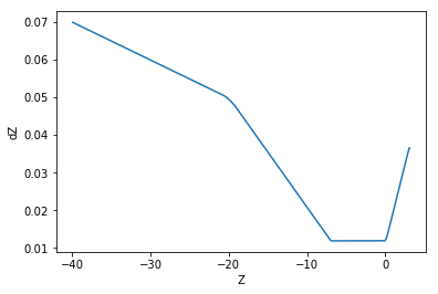
Small Demo

Here, we plot dz versus z, illustrating the non-uniform gaps in the z axis.

from helita.sim import bifrost as br
import matplotlib.pyplot as plt
import numpy as np

rootname='l2d90x40r_it' #this is for the 2D case
fdir='/net/opal/Volumes/Amnesia/mpi3drun/2Druns/genohm/rain/l2d90x40r'
dd=br.BifrostData(rootname,fdir=fdir, verbose = False) #this loads the structure
var=dd.get_var('r',305) #this reads the density (r) for the instant 305

# gets the z coordinates of data points and makes an empty array of the same length for values of dz
zarr = dd.z
length = zarr.shape[0]
dzarr = np.empty([length])

# iterates through zarr and sets each entry in dzarr as the difference between the next and current values of z
# for the final value of dzarr, sets it to be the same as the previous value of dzarr
for i, val in enumerate(zarr):
    if i < length - 1 :
        dzarr[i] = zarr[i + 1] - val
        i = i + 1

    else :
        dzarr[i] = dzarr[i - 1]

# plots z vs dz and labels the axes
plt.plot(zarr, dzarr)
plt.xlabel('Z')
plt.ylabel('dZ')
plt.show()

WARNING: cstagger use has been turned off, turn it back on with "dd.cstagop = True"

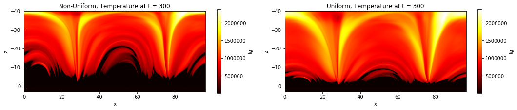
In this example, we interpolate temperature data from the simulation to conform to a uniform z axis and plot the data with both the original, and the even, z axes.

import scipy.interpolate as sp
# bifrost already imported and dd initialized after previous example

temp = dd.get_var('tg', 300)

zarr = dd.z
xarr = dd.x

# at instant 305 -  x is uniform, y is kept constant, and z is non uniform

# converts the 3d array with width of 1 to 2d array (and transposes because otherwise image is sidewise)
temp2d = np.transpose(temp[:,0])

f = sp.interp2d(xarr, zarr, temp2d)

# makes a new uniform z, x is already uniform
zlength = zarr.shape[0]
zstart = zarr[0]
zend = zarr[zlength - 1]
newz = np.linspace(zstart, zend, zlength)

# makes the interpolated data with the previously created interpolation function acting on the new uniform axes
uniform_a = f(xarr, newz)

fig = plt.figure(figsize = (15, 3))

# optional plotting of the non uniform data to show the difference
ax0 = fig.add_subplot(1, 2, 1)
im0 = ax0.imshow(temp2d, cmap = 'hot', extent = (xarr[0], xarr[xarr.shape[0] - 1], zend, zstart), aspect = 'equal')
ax0.set_title('Non-Uniform, Temperature at t = 300')
ax0.set_xlabel('x')
ax0.set_ylabel('z')
c0 = fig.colorbar(im0, ax = ax0)
c0.set_label('tg')

ax1 = fig.add_subplot(1, 2, 2)
im1 = ax1.imshow(uniform_a, cmap = 'hot', extent = (xarr[0], xarr[xarr.shape[0] - 1], zend, zstart), aspect = 'equal')
ax1.set_title('Uniform, Temperature at t = 300')
ax1.set_xlabel('x')
ax1.set_ylabel('z')
c1 = fig.colorbar(im1, ax = ax1)
c1.set_label('tg')
plt.tight_layout()
plt.show()

create_new_br_files class

bifrost_units class

Rhoeetab class

Opatab class

FFTData class

This class can be found within bifrost_fft.py. It performs operations on Bifrost simulation data in its native format. After creating a class for a specific snap root name and directory (much like with BifrostData), one can get a dictionary of the frequency and amplitude of the Fourier Transform for a certain quantity over a range of snapshots.

We have defined 3 variables that allow us to decompose the velocity in Alfvenic, fast mode and longitudinal component (‘alf’, ‘fast’, and ‘long’). Here, we show the transformation of ‘alf’,

from helita.sim import bifrost_fft as brft

dd = brft.FFTData(file_root = 'cb10f', fdir = '/net/opal/Volumes/Amnesia/mpi3drun/Granflux')

transformed = dd.get_fft('alf', snap = [430, 431, 432], iix = 5, iiy = 20)

WARNING: cstagger use has been turned off, turn it back on with "dd.cstagop = True"

transformed.keys()

dict_keys(['freq', 'ftCube'])

Depending on the number of snaps and the size of the cube, using cuda or python multiprocessing may speed up the calculation.

1. Using cuda

If pycuda is available, the code imports reikna (a python library that contains fft functions using pycuda). In order to make use of the GPU, use the function run_gpu(). The default is to not use the GPU, even if there is one available.

dd.run_gpu() # to use GPU
dd.run_gpu(False) # to stop use of GPU

When get_fft() is called, the GPU will be used in accordance with the last call to run_gpu(). If the GPU has limited memory, the user can specify numBlocks in the call to get_fft(). This will send the calculation over to the GPU in several blocks as opposed to all at once. To use 5 different blocks, a call would look like this:

usingBlocks = dd.get_fft('bx', snap = [400, 401, 402], numBlocks = 5)

2. Using python multiprocessing

This can be used whether or not pycuda is available, as multiprocessing is a library that comes with python. It makes use of threading on the CPU. In order to use a multiprocessing threadpool when calculating the Fourier Transform, specify numThreads with a number greater than 1, when calling get_fft():

usingThreads = dd.get_fft('bx', snap = [400, 401, 402], numThreads = 10)

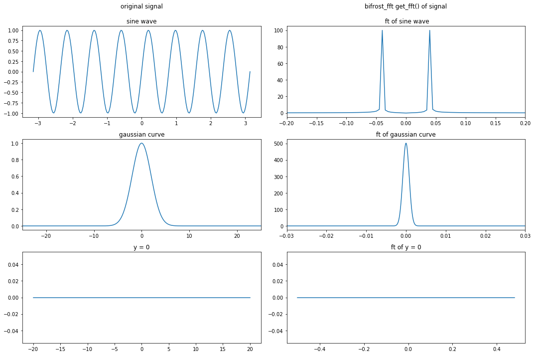
FFT demo #1

This first demo tests the get_fft() method with standard functions: a sine wave, a gaussian curve, and y = 0. It pre-sets dd.preTransform and

import numpy as np
import helita.sim.cstagger
from helita.sim.bifrost import BifrostData, Rhoeetab, read_idl_ascii
from helita.sim.bifrost_fft import FFTData
import matplotlib.pyplot as plt

# note: this calls bifrost_fft from user, not /sanhome

dd = FFTData(file_root='cb10f',
             fdir='/net/opal/Volumes/Amnesia/mpi3drun/Granflux')

# test 1: ft of y = sin(8x)
x = np.linspace(-np.pi, np.pi, 201)
dd.preTransform = np.sin(8 * x)
dd.freq = np.fft.fftshift(np.fft.fftfreq(np.size(x)))
dd.run_gpu(False)
# preTransform is already set
tester = dd.get_fft('not a real var', snap='test')
fig = plt.figure(figsize=(15,10))

numC = 3
numR = 2

# plotting original sin signal
ax0 = fig.add_subplot(numC, numR, 1)
ax0.plot(x, dd.preTransform)
ax0.set_title('original signal' + '\n\nsine wave')

# plotting transformation sin signal
ax1 = fig.add_subplot(numC, numR, 2)
ax1.plot(tester['freq'], tester['ftCube'])
ax1.set_title('bifrost_fft get_fft() of signal' + '\n\n ft of sine wave')
ax1.set_xlim(-.2, .2)

# test 2: ft of gaussian curve
n = 30000  # Number of data points
dx = .01  # Sampling period (in meters)
x = dx*np.linspace(-n/2, n/2, n)  # x coordinates

stanD = 2  # standard deviation
dd.preTransform = np.exp(-0.5 * (x/stanD)**2)

# plotting original gaussian signal
ax2 = fig.add_subplot(numC, numR, 3)
ax2.plot(x, dd.preTransform)
ax2.set_xlim(-25, 25)
ax2.set_title('gaussian curve')

# plotting transformation of gaussian signal
dd.freq = np.fft.fftshift(np.fft.fftfreq(np.size(x)))
ft = dd.get_fft('not a real var', snap='test')  # preTransform is already set
ax3 = fig.add_subplot(numC, numR, 4)
ax3.plot(ft['freq'], ft['ftCube'])
ax3.set_xlim(-.03, .03)
ax3.set_title('ft of gaussian curve')

# test 3: ft of y = 0
# plotting original horizontal line
x = np.linspace(-20, 20, 50)
dd.preTransform = [0] * 50
ax4 = fig.add_subplot(numC, numR, 5)
ax4.plot(x, dd.preTransform)
ax4.set_title('y = 0')

# plotting transformed signal
dd.freq = np.fft.fftshift(np.fft.fftfreq(np.size(x)))
ft = dd.get_fft('not a real var', snap='test')  # preTransform is already set
ax5 = fig.add_subplot(numC, numR, 6)
ax5.plot(ft['freq'], ft['ftCube'])
ax5.set_title('ft of y = 0')

plt.tight_layout()
plt.show()

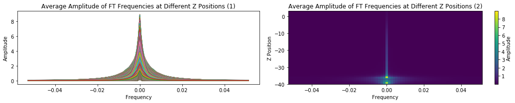
FFT demo #2

Here, we use get_fft() to find the transformation result for bx at each z position (from a local network containing 2d simulations).

import numpy as np
import helita.sim.cstagger
from helita.sim.bifrost import BifrostData, Rhoeetab, read_idl_ascii
from helita.sim.bifrost_fft import FFTData
import matplotlib.pyplot as plt

snaps = np.arange(280, 360)
v = 'bx'

dd = FFTData(file_root='l2d90x40r_it',
             fdir='/net/opal/Volumes/Amnesia/mpi3drun/2Druns/genohm/rain/l2d90x40r/')

# getting ft
transformed = dd.get_fft(v, snaps)
ft = transformed['ftCube']
freq = transformed['freq']
zaxis = dd.z

# making empty array to later contain the avergaes for each z position
zstack = np.empty([np.size(freq), np.shape(ft)[1]])
# filling ztack with average ft for each (x,y) in each z level
for k in range(0, np.shape(ft)[1]):
    avg = np.average(ft[:, k, :], axis=(0))
    zstack[:, k] = avg

# preparing plots
fig = plt.figure(figsize = (15, 3))
numC = 1
numR = 2

# ploting freq vs amp with multiple lines (1 for each z position)
ax0 = fig.add_subplot(numC, numR, 1)
ax0.plot(freq, zstack)
ax0.set_xlabel('Frequency')
ax0.set_ylabel('Amplitude')
ax0.set_title(
    'Average Amplitude of FT Frequencies at Different Z Positions (1)')
ax0.set_aspect('auto')

# plotting amp at different freq & z with image
ax1 = fig.add_subplot(numC, numR, 2)
im1 = ax1.imshow(zstack.transpose(), extent=[freq[0], freq[-1], zaxis[0], zaxis[-1]])
ax1.set_xlabel('Frequency')
ax1.set_ylabel('Z Position')
ax1.set_title(
    'Average Amplitude of FT Frequencies at Different Z Positions (2)')
ax1.set_aspect('auto')
c1 = fig.colorbar(im1, ax = ax1)
c1.set_label('Amplitude')
plt.tight_layout()
plt.show()

WARNING: cstagger use has been turned off, turn it back on with "dd.cstagop = True"