bq_t5_look tool
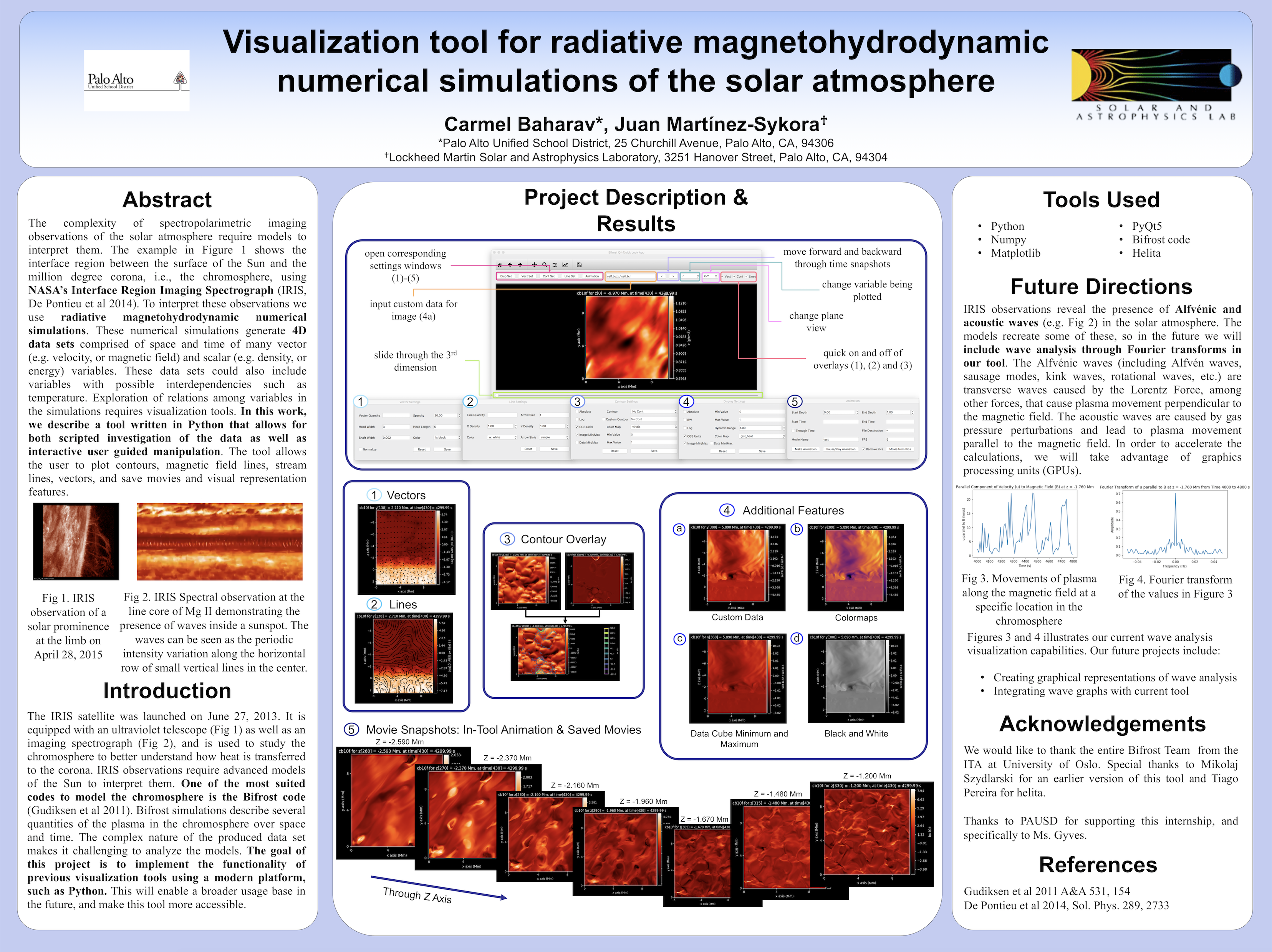
This tool can be used to visualize and manipulate data sets produced by Bifrost (and Ebysus) simulations. Previous tools were written in IDL, but this tool is written in Python, increasing accessibility. It also has a range of added features including the creation of movies and animations.
Poster submitted to AGU Virtual Poster Showcase Fall of 2017
Setup
Note
The Bifrost code, which includes this tool, is not publicly available yet.
This tool can be found in Bifrost (which is a separate folder from helita), and requires that helita be installed in order to function. Once you have created a path for the Bifrost folder, add that path to your .cshrc, eg:
setenv BIFROSTPATH yourpath
Launch
To launch the tool, call:
python path_to_file -i path_to_snapshot
Possible extensions include:
| -i, --input | required, points to snapshot file |
| -h, --help | returns help message |
| -s, --slice | jumps directly to data[:, :, slice], defaults to 0 |
| -z, --depth | finds a slice at the corresponding depth value provided in real [mM] coordinates |
| -e, --ebysus | code based on Bifrost |
Description
Initial window
- Slider: moves through third dimension
- Variable choice: select variable to be plotted from dropdown
- Customizable quantity: input custom data for image
- Plane view: select plane view from dropdown
- Control of overlays: quickly add or remove overlays specified in respective window
Overlays & additional settings
Each of the overlays (vectors, lines, and contour) has its own corresponding pop-up settings window that can be opened from the initial page of the tool. As previously mentioned, the initial window also has the option to quickly hide/reveal a previously loaded overlay. By default, all overlays are shown once a quantity is specified.
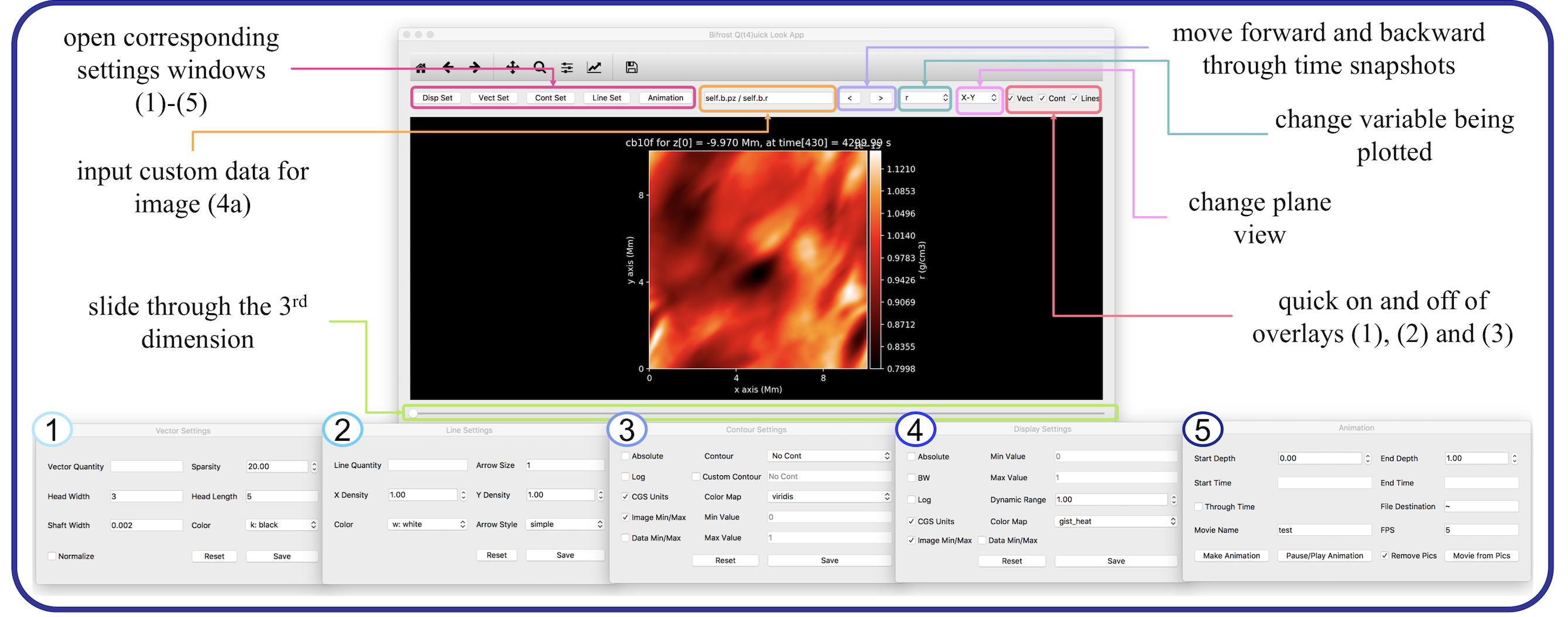
1. Vectors
Vector Settings Window
- This feature allows the user to visualize non-scalar data. The user can manipulate:
- Vector quantity (eg. p or u)
- Arrow head width/length
- Arrow shaft width
- Sparsity of vectors shown
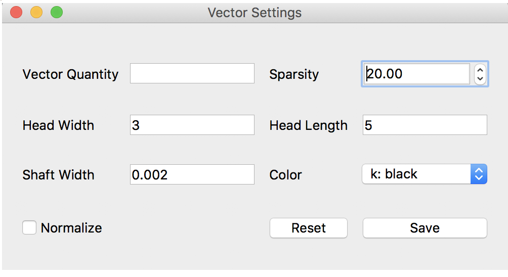
2. Lines
Line Settings Window
- Lines offer the user another method of illustrating non-scalar data besides vector fields. The user can specify:
- Line quantity (eg. b)
- Line density in the X and Y directions
- Line color
- Arrow style and size
3. Contour
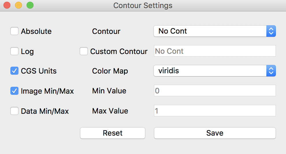
Contour Settings Window
- Plotting contours allows the user to display two scalar quantities simultaneously. The user can determine:
- Contour quantity (can select from dropdown or specify custom quantity)
- Scale (eg. absolute or log)
- Units (CGS)
- Minimum and maximum used (based on individual slice, whole data cube, or custom values)
- Color map
4. Additional display features
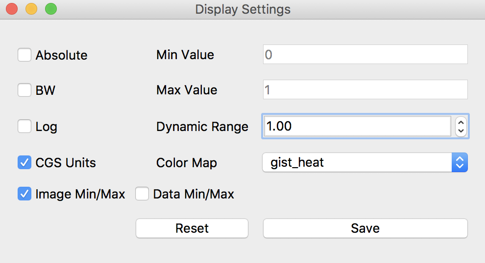
Display Settings Window
- These settings alter the background image and provide similar options to the contour settings. The added specifications are:
- Black and white image
- Dynamic range
- The repeated features are:
- Scale
- Units
- Minimum and maximum used
- Color Map
5. Movies and animation
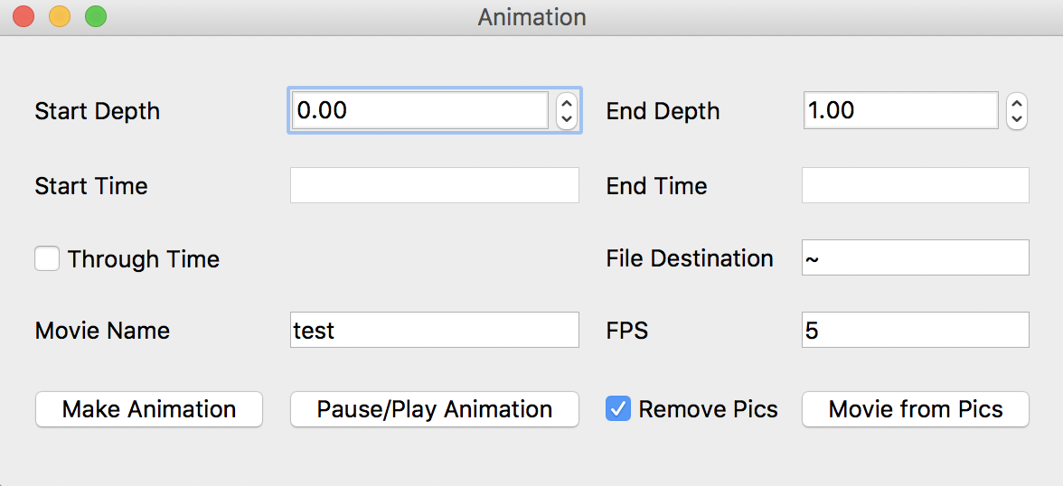
Animation Settings Window
- Both animations and movies use the current settings (including any overlays that are active), and can move through either time or space. With both, the user can specify:
- Start depth and end depth
- OR start time and end time (if “Through Time” box is checked)
- Animation features:
- Make animation begins the animation on the display window
- User can pause/play current animation at any point
- Animation will loop until paused
- Movie features:
- File destination (default is home directory)
- Frames per second
- Whether pictures should be saved or removed (the movie is created from saved pictures)